Visualizations¶

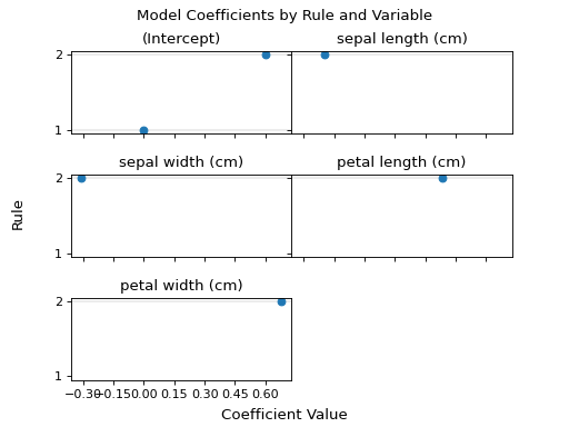
Cubist Coefficient Display¶

class cubist.cubist_coefficient_display.CubistCoefficientDisplay(*, coeffs: DataFrame)[source]¶

Visualization of the regression coefficients used in the Cubist model.

This tool plots the linear coefficients and intercepts created for a Cubist model and stored in the coeffs_ attribute. One subplot is created for each variable or intercept with the rule number or committee/rule pair on the y-axis. The coefficient values for the given variable and rule pair or variable and committee/rule pair are plotted along the x-axis.

See the details in the docstrings of from_estimator() to create a visualizer. All parameters are stored as attributes.

Added in version 1.0.0.

Parameters:

coeffspd.DataFrame: DataFrame containing the linear model coefficients by variable, committee, and rule.

Attributes:

ax_matplotlib Axes: Axes with the different matplotlib axis.
figure_matplotlib Figure: Figure containing the scatter and lines.

See also

CubistCoefficientDisplay.from_estimator: Plot the coefficients used in the Cubist model.

Examples

>>> import matplotlib.pyplot as plt
>>> from sklearn.datasets import load_iris
>>> from cubist import Cubist, CubistCoefficientDisplay
>>> X, y = load_iris(return_X_y=True, as_frame=True)
>>> model = Cubist(n_rules=2).fit(X, y)
>>> display = CubistCoefficientDisplay.from_estimator(estimator=model)
>>> plt.show()

plot(ax=None, y_label_map: dict = None, *, y_axis_label: str = None, gridspec_kwargs: dict = None, scatter_kwargs: dict = None)[source]¶

Plot visualization.

Extra keyword arguments will be passed to matplotlib’s subplots and scatter.

Parameters:

axmatplotlib axes, default=None: Axes object to plot on. If None, a new figure and axes is created.
y_label_mapdict, default=None: Dictionary mapping ordered value to the y-axis tick label so that matplotlib correctly orders committee/rule pairs in addition to rule numbers along the y-axis.
y_axis_labelstr, default=None: Y-axis label for plot.
**gridspec_kwargsdict: Additional keywords arguments passed to matplotlib matplotlib.pyplot.subplots function.
**scatter_kwargsdict: Additional keywords arguments passed to matplotlib matplotlib.pyplot.scatter function.

Returns:

displayCubistCoefficientDisplay: Object that stores computed values.

classmethod from_estimator(estimator: Cubist, *, committee: int = None, rule: int = None, feature_names: list = None, ax=None, scatter_kwargs=None, gridspec_kwargs=None)[source]¶

Plot the coefficients used in the Cubist model.

Added in version 1.0.0.

Parameters:

estimatorCubist instance: Fitted Cubist regressor.
committeeint: Max committee number to be included in plot.
ruleint: Max rule number to be included in plot.
feature_nameslist of str: Feature names to filter to in the plot. Leaving unset plots all features.
axmatplotlib axes, default=None: Axes object to plot on. If None, a new figure and axes is created.
scatter_kwargsdict, default=None: Dictionary with keywords passed to the matplotlib.pyplot.scatter call.
gridspec_kwargsdict, default=None: Dictionary with keyword passed to the matplotlib.pyplot.subplots call to configure the subplot.

Returns:

displayCubistCoefficientDisplay: Object that stores the computed values.

See also

CubistCoefficientDisplay: Cubist coefficient visualization.

Examples

>>> import matplotlib.pyplot as plt
>>> from sklearn.datasets import load_iris
>>> from cubist import Cubist, CubistCoefficientDisplay
>>> X, y = load_iris(return_X_y=True, as_frame=True)
>>> model = Cubist(n_rules=2).fit(X, y)
>>> display = CubistCoefficientDisplay.from_estimator(estimator=model)
>>> plt.show()

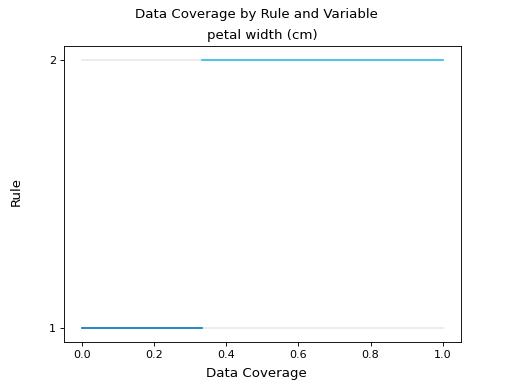
Cubist Coverage Display¶

class cubist.cubist_coverage_display.CubistCoverageDisplay(*, splits: DataFrame)[source]¶

Visualization of rule split coverage for input variables for a trained Cubist model.

This tool plots the percents and ranges (coverage) per rule of input variables from a given dataset. One subplot is created for each variable used to make splits with the rule number or committee/rule pair on the y-axis. The coverage percentages for the given variable and rule pair or variable and committee/rule pair are plotted along the x-axis.

See the details in the docstrings of from_estimator() to create a visualizer. All parameters are stored as attributes.

Added in version 1.0.0.

Parameters:

splitspd.DataFrame: DataFrame containing the model split values by variable, committee, and rule.

Attributes:

ax_matplotlib Axes: Axes with the different matplotlib axis.
figure_matplotlib Figure: Figure containing the scatter and lines.

See also

CubistCoverageDisplay.from_estimator: Cubist input variable coverage visualization.

Examples

>>> import matplotlib.pyplot as plt
>>> from sklearn.datasets import load_iris
>>> from cubist import Cubist, CubistCoverageDisplay
>>> X, y = load_iris(return_X_y=True, as_frame=True)
>>> model = Cubist(n_rules=2).fit(X, y)
>>> display = CubistCoverageDisplay.from_estimator(estimator=model, X=X)
>>> plt.show()

plot(ax=None, y_label_map: dict = None, *, y_axis_label: str = None, gridspec_kwargs: dict = None, line_kwargs: dict = None)[source]¶

Plot visualization.

Extra keyword arguments will be passed to matplotlib’s subplots and plot.

Parameters:

axmatplotlib axes, default=None: Axes object to plot on. If None, a new figure and axes is created.
y_label_mapdict, default=None: Dictionary mapping ordered value to the y-axis tick label so that matplotlib correctly orders committee/rule pairs in addition to rule numbers along the y-axis.
y_axis_labelstr, default=None: Y-axis label for plot.
**gridspec_kwargsdict: Additional keywords arguments passed to matplotlib matplotlib.pyplot.subplots function.
**line_kwargsdict: Additional keywords arguments passed to matplotlib matplotlib.pyplot.plot function.

Returns:

displayCubistCoverageDisplay: Object that stores computed values.

classmethod from_estimator(estimator: Cubist, X, *, committee: int = None, rule: int = None, feature_names: list = None, ax=None, line_kwargs=None, gridspec_kwargs=None)[source]¶

Plot the input variable coverage for rules used in the Cubist model.

Added in version 1.0.0.

Parameters:

estimatorCubist instance: Fitted Cubist regressor.
Xarray-like of shape (n_samples, n_features): Training data, where n_samples is the number of samples and n_features is the number of features.
committeeint: Max committee number to be included in plot.
ruleint: Max rule number to be included in plot.
feature_nameslist of str: Feature names to filter to in the plot. Leaving unset plots all features.
axmatplotlib axes, default=None: Axes object to plot on. If None, a new figure and axes is created.
line_kwargsdict, default=None: Dictionary with keywords passed to the matplotlib.pyplot.plot call.
gridspec_kwargsdict, default=None: Dictionary with keyword passed to the matplotlib.pyplot.subplots call to configure the subplot.

Returns:

displayCubistCoverageDisplay: Object that stores the computed values.

See also

CubistCoverageDisplay: Cubist input variable coverage visualization.

Examples

>>> import matplotlib.pyplot as plt
>>> from sklearn.datasets import load_iris
>>> from cubist import Cubist, CubistCoverageDisplay
>>> X, y = load_iris(return_X_y=True, as_frame=True)
>>> model = Cubist(n_rules=2).fit(X, y)
>>> display = CubistCoverageDisplay.from_estimator(estimator=model, X=X)
>>> plt.show()